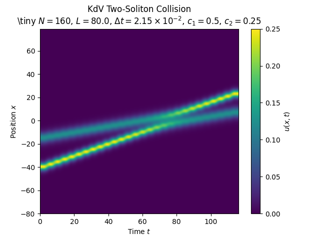
Space-Time Visualization for Two-Soliton Collision

Creates space-time visualization showing the full evolution of the two-soliton collision in the KdV equation.

Imports

We start by importing the necessary libraries and utility functions.

import numpy as np
import pandas as pd
import matplotlib.pyplot as plt

from spectral.utils.plotting import get_repo_root
from spectral.utils.io import ensure_output_dir
from spectral.utils.formatting import extract_metadata, format_dt_latex

Load simulation data

Load the two-soliton collision dataset generated by compute.py. This contains the solution u(x,t) at regularly saved time snapshots.

repo_root = get_repo_root()
data_dir = repo_root / "data/A2/ex_f"
save_dir = ensure_output_dir(repo_root / "figures/A2/ex_f")

print("=" * 60)
print("Exercise f – two-soliton collision (space-time plot)")
print("=" * 60)

df = pd.read_parquet(data_dir / "kdv_two_soliton.parquet")
print(f"Data shape: {df.shape}")

preferred_treatments = [
    "De-aliased (3/2-rule)",
    "Aliased",
]

if "Treatment" in df.columns:
    available = list(df["Treatment"].drop_duplicates())
    print(f"Available treatments: {available}")
    target_treatment = None
    for candidate in preferred_treatments:
        if candidate in available:
            target_treatment = candidate
            break
    if target_treatment is None and available:
        target_treatment = available[0]
    if target_treatment:
        df = df[df["Treatment"] == target_treatment].copy()
        print(f"Selected treatment for plotting: {target_treatment}")

============================================================
Exercise f – two-soliton collision (space-time plot)
============================================================
Data shape: (8960, 14)
Available treatments: ['Aliased', 'De-aliased (3/2-rule)']
Selected treatment for plotting: De-aliased (3/2-rule)

Extract metadata

The dataset contains simulation parameters like grid spacing, time step, and soliton speeds that we’ll need for the plot annotations.

metadata = extract_metadata(
    df, ["dx", "dt", "N", "L", "save_every", "c1", "x01", "c2", "x02"]
)

print("Metadata:")
for key, val in metadata.items():
    print(f"  {key} = {val}")

Metadata:
  dx = 1.0
  dt = 0.02151073139005624
  N = 160
  L = 80.0
  save_every = 200
  c1 = 0.5
  x01 = -40.0
  c2 = 0.25
  x02 = -15.0

Reshape to grid

The data is stored in tidy format. For visualization, we need to reshape it into a 2D grid (x, t). We also downsample to reduce the file size while keeping endpoints for accuracy.

x_vals = np.sort(df["x"].unique())
t_vals = np.sort(df["t"].unique())

print(f"Unique x count: {len(x_vals)}, unique t count: {len(t_vals)}")


def _select_indices(n: int, max_points: int) -> np.ndarray:
    """Return indices that downsample to at most max_points while keeping endpoints."""
    if max_points <= 0 or n <= max_points:
        return np.arange(n, dtype=int)
    stride = int(np.ceil(n / max_points))
    idx = np.arange(0, n, stride, dtype=int)
    if idx[-1] != n - 1:
        idx = np.append(idx, n - 1)
    return idx


max_x_points = 400
max_t_points = 800

idx_x = _select_indices(len(x_vals), max_x_points)
idx_t = _select_indices(len(t_vals), max_t_points)

df_matrix = df.pivot(index="x", columns="t", values="u")
df_matrix = df_matrix.reindex(index=x_vals, columns=t_vals)
df_down = df_matrix.iloc[idx_x, idx_t]
x_plot = df_down.index.to_numpy()
t_plot = df_down.columns.to_numpy()

Unique x count: 160, unique t count: 28

Create space-time plot

Visualize the full space-time evolution as a heatmap. The collision of the two solitons is clearly visible, as well as the characteristic phase shift that occurs during the interaction.

fig, ax = plt.subplots()
im = ax.imshow(
    df_down.values,
    aspect="auto",
    origin="lower",
    extent=[t_plot[0], t_plot[-1], x_plot[0], x_plot[-1]],
)
fig.colorbar(im, ax=ax, label=r"$u(x, t)$")

ax.set_xlabel(r"Time $t$")
ax.set_ylabel(r"Position $x$")
N = metadata.get("N", "?")
L = metadata.get("L", "?")
dt = metadata.get("dt", "?")
c1 = metadata.get("c1", "?")
c2 = metadata.get("c2", "?")
dt_latex = format_dt_latex(dt)
ax.set_title(
    "KdV Two-Soliton Collision"
    + "\n"
    + rf"\tiny $N = {N}$, $L = {L}$, $\Delta t = {dt_latex}$, $c_1 = {c1}$, $c_2 = {c2}$",
)

output_path = save_dir / "spacetime.pdf"
fig.savefig(output_path, bbox_inches="tight")
print(f"Saved space-time plot → {output_path}")

print("=" * 60)
print("Plotting complete.")
print("=" * 60)

Saved space-time plot → /home/docs/checkouts/readthedocs.org/user_builds/02689-advanced-num-alg/checkouts/latest/figures/A2/ex_f/spacetime.pdf
============================================================
Plotting complete.
============================================================