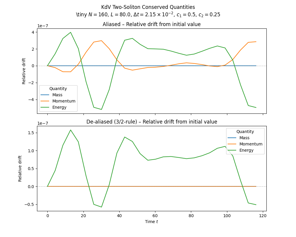
Conserved Quantities for Two-Soliton Collision

Plots conserved quantities (mass, momentum, energy) for the two-soliton collision in the KdV equation.

Conservation laws Visualize conservation of mass, momentum, and energy.

import numpy as np
import pandas as pd
import matplotlib.pyplot as plt
import seaborn as sns

from spectral.tdp import KdVSolver
from spectral.utils.plotting import get_repo_root
from spectral.utils.io import load_simulation_data, ensure_output_dir
from spectral.utils.formatting import extract_metadata, format_dt_latex

TREATMENT_ORDER = ["Aliased", "De-aliased (3/2-rule)"]
QUANTITY_ORDER = ["Mass", "Momentum", "Energy"]


repo_root = get_repo_root()
data_dir = repo_root / "data/A2/ex_f"
save_dir = ensure_output_dir(repo_root / "figures/A2/ex_f")

print("=" * 60)
print("Exercise f – two-soliton invariants")
print("=" * 60)

============================================================
Exercise f – two-soliton invariants
============================================================

df = load_simulation_data(data_dir, "kdv_two_soliton")
print(f"Data shape: {df.shape}")

if "Treatment" not in df.columns:
    df["Treatment"] = "Aliased"
if "dealias" not in df.columns:
    df["dealias"] = df["Treatment"].eq("De-aliased (3/2-rule)")

# Metadata
metadata = extract_metadata(
    df, ["dx", "dt", "N", "L", "save_every", "c1", "x01", "c2", "x02"]
)

print("Metadata:")
for key, val in metadata.items():
    print(f"  {key} = {val}")

available_treatments = list(df["Treatment"].drop_duplicates())
print(f"Treatments present: {available_treatments}")

Loading parquet data: /home/docs/checkouts/readthedocs.org/user_builds/02689-advanced-num-alg/checkouts/latest/data/A2/ex_f/kdv_two_soliton.parquet
Data shape: (8960, 14)
Metadata:
  dx = 1.0
  dt = 0.02151073139005624
  N = 160
  L = 80.0
  save_every = 200
  c1 = 0.5
  x01 = -40.0
  c2 = 0.25
  x02 = -15.0
Treatments present: ['Aliased', 'De-aliased (3/2-rule)']

Sort to ensure deterministic ordering within each (Treatment, t)

df_sorted = df.sort_values(["Treatment", "t", "x"])


def _compute_quantities(group: pd.DataFrame) -> pd.Series:
    if "dx" in group.columns:
        dx_local = float(group["dx"].iloc[0])
    else:
        x_vals_local = np.sort(group["x"].unique())
        if len(x_vals_local) > 1:
            dx_local = float(np.diff(x_vals_local).mean())
        else:
            dx_local = 1.0
    M, V, E = KdVSolver.compute_conserved_quantities(group["u"].to_numpy(), dx_local)
    return pd.Series({"Mass": M, "Momentum": V, "Energy": E})


df_abs = (
    df_sorted.groupby(["Treatment", "t"], sort=False, observed=True)
    .apply(_compute_quantities, include_groups=False)
    .reset_index()
)

df_abs["Treatment"] = pd.Categorical(
    df_abs["Treatment"], categories=TREATMENT_ORDER, ordered=True
)

df_rel = df_abs.copy()
grouped_rel = df_rel.groupby("Treatment", sort=False, observed=True)
for quantity in QUANTITY_ORDER:
    df_rel[quantity] = grouped_rel[quantity].transform(
        lambda series: (series - series.iloc[0]) / (abs(series.iloc[0]) or 1.0)
    )

df_rel_long = df_rel.melt(
    id_vars=["Treatment", "t"],
    value_vars=QUANTITY_ORDER,
    var_name="Quantity",
    value_name="Relative drift",
)
df_rel_long["Quantity"] = pd.Categorical(
    df_rel_long["Quantity"], categories=QUANTITY_ORDER, ordered=True
)

fig, axs = plt.subplots(
    2, 1, figsize=(10, 8), sharex=True, gridspec_kw={"hspace": 0.15}
)

for ax, treatment in zip(axs, TREATMENT_ORDER):
    subset = df_rel_long[df_rel_long["Treatment"] == treatment]
    if subset.empty:
        ax.set_visible(False)
        continue
    sns.lineplot(
        data=subset,
        x="t",
        y="Relative drift",
        hue="Quantity",
        hue_order=QUANTITY_ORDER,
        ax=ax,
    )
    ax.axhline(0.0, color="gray", linestyle="--", linewidth=0.8, alpha=0.6)
    ax.set_ylabel("Relative drift")
    ax.set_title(f"{treatment} – Relative drift from initial value")
    ax.legend(loc="best", title="Quantity")

axs[-1].set_xlabel(r"Time $t$")

# Add overall title with parameters
N = metadata.get("N", "?")
L = metadata.get("L", "?")
dt = metadata.get("dt", "?")
c1 = metadata.get("c1", "?")
c2 = metadata.get("c2", "?")
dt_latex = format_dt_latex(dt)
fig.suptitle(
    "KdV Two-Soliton Conserved Quantities"
    + "\n"
    + rf"\tiny $N = {N}$, $L = {L}$, $\Delta t = {dt_latex}$, $c_1 = {c1}$, $c_2 = {c2}$",
    y=0.98,
)

output_path = save_dir / "invariants.pdf"
fig.savefig(output_path, bbox_inches="tight")
print(f"Saved invariants plot → {output_path}")

print("=" * 60)
print("Invariant plotting complete.")
print("=" * 60)

Saved invariants plot → /home/docs/checkouts/readthedocs.org/user_builds/02689-advanced-num-alg/checkouts/latest/figures/A2/ex_f/invariants.pdf
============================================================
Invariant plotting complete.
============================================================