KdV Solutions - Separate plots per method

Creates separate visualization panels for each time integration method (RK4, RK3) showing soliton propagation.

Kdv solutions Visualize soliton propagation for different time integrators.

import numpy as np
import pandas as pd
import seaborn as sns

from spectral.utils.plotting import get_repo_root
from spectral.utils.io import ensure_output_dir
from spectral.utils.formatting import format_dt_latex

repo_root = get_repo_root()
data_dir = repo_root / "data/A2/ex_c"
save_dir = ensure_output_dir(repo_root / "figures/A2/ex_c")

print("Loading KdV solutions data...")
df = pd.read_parquet(data_dir / "kdv_solutions.parquet")

print(f"  Data shape: {df.shape}")
print(f"  Methods: {sorted(df['method'].unique())}")
print(f"  c values: {sorted(df['c'].unique())}")
print(f"  N values: {sorted(df['N'].unique())}")

# Filter for largest N
largest_N = df["N"].max()
df = df[df["N"] == largest_N].copy()
print(f"\nFiltered to largest N = {largest_N}")
print(f"  Filtered data shape: {df.shape}")

Loading KdV solutions data...
  Data shape: (947800, 12)
  Methods: ['RK3', 'RK4']
  c values: [0.25, 0.5, 1.0]
  N values: [200]

Filtered to largest N = 200
  Filtered data shape: (947800, 12)

for method in sorted(df["method"].unique()):
    print(f"\nProcessing method: {method}")

    df_method = df[df["method"] == method].copy()

    # Get smallest dt for each c value and select timesteps independently
    df_method_filtered = []
    for c_val in sorted(df_method["c"].unique()):
        df_c = df_method[df_method["c"] == c_val].copy()
        unique_dt_c = sorted(df_c["dt"].unique())
        smallest_dt_c = unique_dt_c[0]
        df_c_filtered = df_c[df_c["dt"] == smallest_dt_c].copy()

        # Select 3 equally spaced timesteps for this c value
        t_vals_c = sorted(df_c_filtered["t"].unique())
        n_times_c = len(t_vals_c)
        indices_c = np.linspace(0, n_times_c - 1, 3, dtype=int)
        selected_t_c = [t_vals_c[i] for i in indices_c]

        # Filter to selected times for this c
        df_c_filtered = df_c_filtered[df_c_filtered["t"].isin(selected_t_c)].copy()

        df_method_filtered.append(df_c_filtered)
        print(
            f"  c={c_val}: using dt = {smallest_dt_c:.6f}, timesteps = {[f'{t:.2f}' for t in selected_t_c]}"
        )

    df_method = pd.concat(df_method_filtered, ignore_index=True)

    # Create time labels
    df_method["Time"] = df_method["t"].apply(lambda t: f"t={t:.1f}")

    # Reshape data to have both numerical and exact solution in long format
    df_numerical = df_method[["x", "u", "t", "c", "Time"]].copy()
    df_numerical["Solution"] = "Numerical"
    df_numerical = df_numerical.rename(columns={"u": "value"})

    df_exact = df_method[["x", "u_exact", "t", "c", "Time"]].copy()
    df_exact["Solution"] = "Exact"
    df_exact = df_exact.rename(columns={"u_exact": "value"})

    df_plot = pd.concat([df_numerical, df_exact], ignore_index=True)

    # Create relplot
    print("  Creating plot...")
    g = sns.relplot(
        data=df_plot,
        x="x",
        y="value",
        hue="Time",
        style="Solution",
        col="c",
        kind="line",
        dashes={"Numerical": "", "Exact": (2, 2)},
        alpha=0.8,
        facet_kws={"legend_out": True},
    )

    # Customize
    g.set_axis_labels(r"Position $x$", r"Amplitude $u$")
    L = df_method["x"].max() - df_method["x"].min()
    dt_min = df_method["dt"].min()
    dt_latex = format_dt_latex(dt_min)
    g.fig.suptitle(f"KdV Solitons - {method}", y=1.05)
    # Escape curly braces in dt_latex for format string
    dt_latex_escaped = dt_latex.replace("{", "{{").replace("}", "}}")
    g.set_titles(
        col_template=r"$c$ = {col_name}"
        + "\n"
        + rf"\tiny $N = {largest_N}$, $L = {L:.1f}$, $\Delta t = {dt_latex_escaped}$"
    )

    # Save
    output = save_dir / f"solutions_{method.lower()}.pdf"
    g.savefig(output)
    print(f"  Saved: {output}")

print("\nAll plots created!")

• 
• 

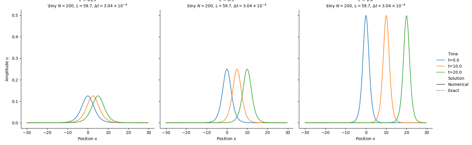
Processing method: RK3
  c=0.25: using dt = 0.000304, timesteps = ['0.00', '9.99', '19.98']
  c=0.5: using dt = 0.000306, timesteps = ['0.00', '9.97', '19.97']
  c=1.0: using dt = 0.000310, timesteps = ['0.00', '9.99', '19.97']
  Creating plot...
  Saved: /home/docs/checkouts/readthedocs.org/user_builds/02689-advanced-num-alg/checkouts/latest/figures/A2/ex_c/solutions_rk3.pdf

Processing method: RK4
  c=0.25: using dt = 0.000496, timesteps = ['0.00', '9.97', '19.99']
  c=0.5: using dt = 0.000499, timesteps = ['0.00', '9.99', '19.97']
  c=1.0: using dt = 0.000506, timesteps = ['0.00', '9.98', '19.95']
  Creating plot...
  Saved: /home/docs/checkouts/readthedocs.org/user_builds/02689-advanced-num-alg/checkouts/latest/figures/A2/ex_c/solutions_rk4.pdf

All plots created!