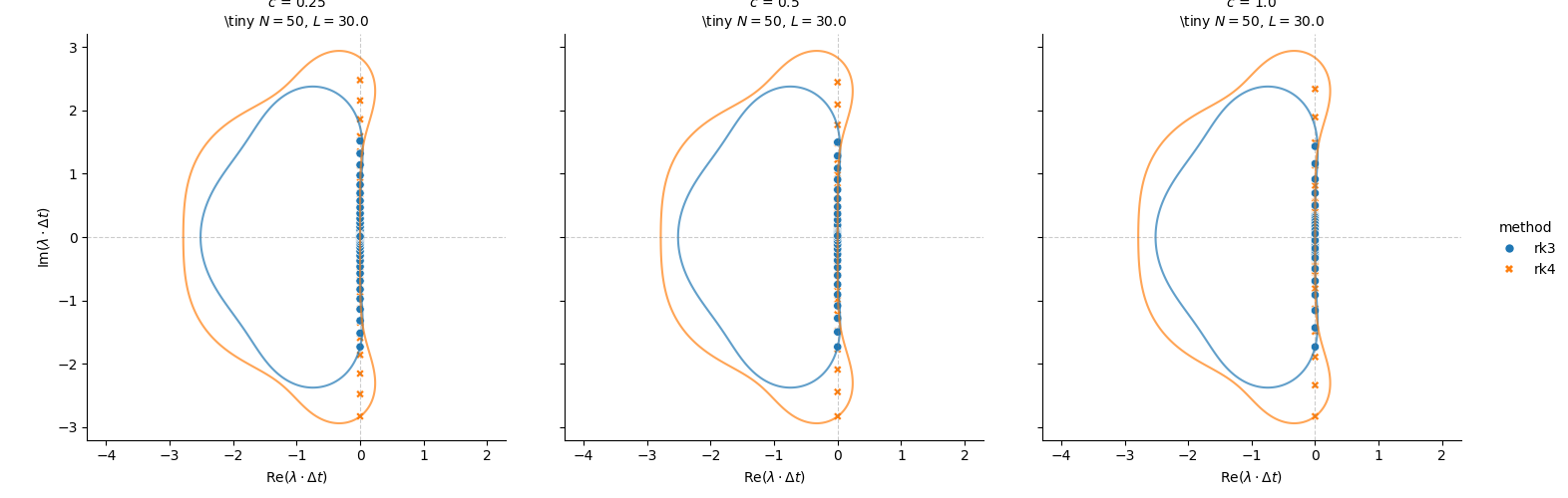
KdV Eigenvalue Stability Analysis - Plotting#

Visualizes eigenvalue stability analysis for different time integrators used in the KdV solver.

Eigenvalue stability analysis Visualize eigenvalue stability regions for different time integrators.

import numpy as np
import pandas as pd
import seaborn as sns

from spectral.utils.plotting import get_repo_root

repo_root = get_repo_root()
data_dir = repo_root / "data/A2/ex_c"
save_dir = repo_root / "figures/A2/ex_c"
save_dir.mkdir(parents=True, exist_ok=True)

print("Loading eigenvalue stability data...")
stability_df = pd.read_parquet(data_dir / "eigenvalue_stability.parquet")
scaling_df = pd.read_parquet(data_dir / "eigenvalue_scaling.parquet")

print(f"  Stability data: {stability_df.shape}")
print(f"  Scaling data: {scaling_df.shape}")

Loading eigenvalue stability data...
  Stability data: (300, 10)
  Scaling data: (24, 8)

print("\nCreating eigenvalue stability plots...")

# Filter finite values
stability_df_finite = stability_df[
    np.isfinite(stability_df["eigval_scaled_real"])
    & np.isfinite(stability_df["eigval_scaled_imag"])
].copy()

# Stability polynomials for linear test eq. u' = λu
R = {
    "rk4": lambda z: 1
    + z
    + 0.5 * z**2
    + (1 / 6) * z**3
    + (1 / 24) * z**4,  # classic RK4
    "rk3": lambda z: 1 + z + 0.5 * z**2 + (1 / 6) * z**3,  # classic/SSP RK3
}

# Create grid showing full stability regions
xmin, xmax = -4.3, 2.3
ymin, ymax = -3.2, 3.2
nx = ny = 800
X, Y = np.meshgrid(np.linspace(xmin, xmax, nx), np.linspace(ymin, ymax, ny))
Z = X + 1j * Y

# Create faceted plot using relplot
g = sns.relplot(
    data=stability_df_finite,
    x="eigval_scaled_real",
    y="eigval_scaled_imag",
    hue="method",
    style="method",
    col="c",
    kind="scatter",
    facet_kws={"sharex": True, "sharey": True},
)

# Add stability regions and formatting to each facet
palette = sns.color_palette(n_colors=len(stability_df["method"].unique()))

for (c_val, method), ax in zip(
    [(c, m) for c in sorted(stability_df["c"].unique()) for m in [None]], g.axes.flat
):
    # Plot stability regions for each method
    for color, m in zip(palette, sorted({s.lower() for s in stability_df["method"]})):
        if m not in R:
            continue
        modR = np.abs(R[m](Z))
        ax.contour(
            X,
            Y,
            modR,
            levels=[1.0],
            colors=[color],
            linestyles="-",
            linewidths=1.5,
            alpha=0.7,
        )

    # Add origin reference
    ax.axhline(y=0, color="gray", linestyle="--", linewidth=0.8, alpha=0.4)
    ax.axvline(x=0, color="gray", linestyle="--", linewidth=0.8, alpha=0.4)
    ax.set_aspect("equal")
    ax.set_xlim(xmin, xmax)
    ax.set_ylim(ymin, ymax)

g.set_axis_labels(r"Re($\lambda \cdot \Delta t$)", r"Im($\lambda \cdot \Delta t$)")
N_stab = stability_df_finite["N"].iloc[0] if "N" in stability_df_finite.columns else 80
L_stab = (
    stability_df_finite["L"].iloc[0] if "L" in stability_df_finite.columns else 30.0
)
g.fig.suptitle(r"KdV Stability", y=1.05)
g.set_titles(r"$c$ = {col_name}" + "\n" + rf"\tiny $N = {N_stab}$, $L = {L_stab:.1f}$")

output = save_dir / "eigenvalue_stability.pdf"
g.savefig(output, bbox_inches="tight")
print(f"  Saved: {output}")

$KdV Stability, $c$ = 0.25 \tiny $N = 50$, $L = 30.0$, $c$ = 0.5 \tiny $N = 50$, $L = 30.0$, $c$ = 1.0 \tiny $N = 50$, $L = 30.0$$

Creating eigenvalue stability plots...
  Saved: /home/docs/checkouts/readthedocs.org/user_builds/02689-advanced-num-alg/checkouts/latest/figures/A2/ex_c/eigenvalue_stability.pdf

# Get unique (c, N) combinations for reference lines
g1 = sns.relplot(
    data=scaling_df.drop_duplicates(["c", "N"]),
    x="N",
    y="max_eigval",
    col="c",
    kind="line",
    markers=True,
    height=4,
    aspect=1.2,
    facet_kws={"sharex": True, "sharey": False},
)

# Add O(N^3) reference line to each facet
for c_val, ax in zip(sorted(scaling_df["c"].unique()), g1.axes.flat):
    c_data = (
        scaling_df[(scaling_df["c"] == c_val)].drop_duplicates("N").sort_values("N")
    )
    N_vals = c_data["N"].values
    max_eigs = c_data["max_eigval"].values
    ax.loglog(
        N_vals,
        (N_vals / N_vals[0]) ** 3 * max_eigs[0],
        "--",
        linewidth=2,
        alpha=0.7,
        label=r"$\mathcal{O}(N^3)$",
        color="gray",
    )
    ax.legend()

g1.set(xscale="log", yscale="log")
g1.set_axis_labels(r"Grid points $N$", r"Maximum $|\lambda|$")
N_min_s = scaling_df["N"].min()
N_max_s = scaling_df["N"].max()
L_s = scaling_df["L"].iloc[0] if "L" in scaling_df.columns else 30.0
g1.fig.suptitle(r"KdV Eigenvalue Scaling", y=1.05)
g1.set_titles(
    r"$c$ = {col_name}"
    + "\n"
    + rf"\tiny $N \in [{N_min_s}, {N_max_s}]$, $L = {L_s:.1f}$"
)

output = save_dir / "eigenvalue_max_scaling.pdf"
g1.savefig(output, bbox_inches="tight")
print(f"  Saved: {output}")

$KdV Eigenvalue Scaling, $c$ = 0.25 \tiny $N \in [32, 256]$, $L = 30.0$, $c$ = 0.5 \tiny $N \in [32, 256]$, $L = 30.0$, $c$ = 1.0 \tiny $N \in [32, 256]$, $L = 30.0$$

Saved: /home/docs/checkouts/readthedocs.org/user_builds/02689-advanced-num-alg/checkouts/latest/figures/A2/ex_c/eigenvalue_max_scaling.pdf

g2 = sns.relplot(
    data=scaling_df,
    x="N",
    y="stable_dt",
    hue="method",
    style="method",
    col="c",
    kind="line",
    markers=True,
    # height=4,
    # aspect=1.2,
    # facet_kws={"sharex": True, "sharey": False},
)

# Add O(N^-3) reference line to each facet
for c_val, ax in zip(sorted(scaling_df["c"].unique()), g2.axes.flat):
    c_data = scaling_df[
        (scaling_df["c"] == c_val) & (scaling_df["method"] == "rk4")
    ].sort_values("N")
    N_vals = c_data["N"].values
    ax.loglog(
        N_vals,
        (N_vals[0] / N_vals) ** 3 * c_data["stable_dt"].iloc[0],
        "--",
        linewidth=2,
        alpha=0.7,
        label=r"$\mathcal{O}(N^{-3})$",
        color="gray",
    )

g2.set(xscale="log", yscale="log")
g2.set_axis_labels(r"Grid points $N$", r"Stable $\Delta t$")
g2.fig.suptitle(r"KdV Timestep Scaling", y=1.05)
g2.set_titles(
    r"$c$ = {col_name}"
    + "\n"
    + rf"\tiny $N \in [{N_min_s}, {N_max_s}]$, $L = {L_s:.1f}$"
)

output = save_dir / "eigenvalue_scaling.pdf"
g2.savefig(output, bbox_inches="tight")
print(f"  Saved: {output}")

print(f"\nAll plots saved to {save_dir}")

$KdV Timestep Scaling, $c$ = 0.25 \tiny $N \in [32, 256]$, $L = 30.0$, $c$ = 0.5 \tiny $N \in [32, 256]$, $L = 30.0$, $c$ = 1.0 \tiny $N \in [32, 256]$, $L = 30.0$$

  Saved: /home/docs/checkouts/readthedocs.org/user_builds/02689-advanced-num-alg/checkouts/latest/figures/A2/ex_c/eigenvalue_scaling.pdf

All plots saved to /home/docs/checkouts/readthedocs.org/user_builds/02689-advanced-num-alg/checkouts/latest/figures/A2/ex_c

Total running time of the script: (0 minutes 2.941 seconds)

Gallery generated by Sphinx-Gallery