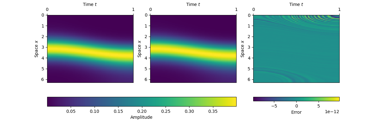
Transport Equation Solutions

Plots transport equation solutions from saved data using Legendre collocation.

Spacetime transport Visualize solutions to the spacetime transport equation.

import numpy as np
import pandas as pd
import matplotlib.pyplot as plt
import seaborn as sns

from spectral.utils.plotting import get_repo_root

repo_root = get_repo_root()
data_dir = repo_root / "data/A2/ex_h"
save_dir = repo_root / "figures/A2/ex_h"
save_dir.mkdir(parents=True, exist_ok=True)

df = pd.read_parquet(data_dir / "solution.parquet")

print(f"Loaded solution data with shape: {df.shape}")
print(f"Columns: {df.columns.tolist()}")
print(f"Types: {df['type'].unique().tolist()}")
print(f"Time points: {df['t'].nunique()}")

Loaded solution data with shape: (30000, 4)
Columns: ['x', 't', 'value', 'type']
Types: ['True', 'Predicted', 'Error']
Time points: 100

xs = np.sort(df["x"].unique())
ts = np.sort(df["t"].unique())

Phi = df[df["type"] == "True"].pivot(index="x", columns="t", values="value").values
Phi_hat = (
    df[df["type"] == "Predicted"].pivot(index="x", columns="t", values="value").values
)
error = df[df["type"] == "Error"].pivot(index="x", columns="t", values="value").values

error_l2 = np.linalg.norm(error)
error_max = np.abs(error).max()

print(f"L2 error: {error_l2:.6e}")
print(f"Max error: {error_max:.6e}")

L2 error: 8.546763e-11
Max error: 9.630825e-12

print("\nCreating heatmap overview...")

fig, axs = plt.subplots(1, 3, figsize=(12, 4))

# Compute color limits for consistent scaling
vmin = min(Phi.min(), Phi_hat.min())
vmax = max(Phi.max(), Phi_hat.max())
errmax = np.abs(error).max()

im0 = axs[0].matshow(
    Phi, vmin=vmin, vmax=vmax, aspect="auto", extent=[ts[0], ts[-1], xs[-1], xs[0]]
)
im1 = axs[1].matshow(
    Phi_hat, vmin=vmin, vmax=vmax, aspect="auto", extent=[ts[0], ts[-1], xs[-1], xs[0]]
)
im2 = axs[2].matshow(
    error,
    cmap="viridis",
    vmin=-errmax,
    vmax=errmax,
    aspect="auto",
    extent=[ts[0], ts[-1], xs[-1], xs[0]],
)

# Colorbars
fig.colorbar(im0, ax=[axs[0], axs[1]], orientation="horizontal", label="Amplitude")
fig.colorbar(im2, ax=axs[2], orientation="horizontal", label="Error")

# Axis formatting
for ax in axs:
    ax.xaxis.tick_top()
    ax.xaxis.set_label_position("top")
    ax.set_xlabel(r"Time $t$")
    ax.set_ylabel(r"Space $x$")

axs[0].set_title("True Solution", pad=20, fontsize=12)
axs[1].set_title("Predicted Solution", pad=20, fontsize=12)
Nx = df["Nx"].iloc[0] if "Nx" in df.columns else len(xs)
Nt = df["Nt"].iloc[0] if "Nt" in df.columns else len(ts)
axs[2].set_title(
    f"Error (L2: {error_l2:.2e})" + "\n" + rf"\tiny $N_x = {Nx}$, $N_t = {Nt}$",
    pad=20,
    fontsize=12,
)

output_path = save_dir / "solution.pdf"
fig.savefig(output_path, dpi=300, bbox_inches="tight")
print(f"Saved: {output_path}")

Creating heatmap overview...
Saved: /home/docs/checkouts/readthedocs.org/user_builds/02689-advanced-num-alg/checkouts/latest/figures/A2/ex_h/solution.pdf

print("\nCreating spatial convergence plot...")

df_spatial = pd.read_parquet(data_dir / "spatial_convergence.parquet")

# Clean up error type labels for display
df_spatial["Error Type"] = df_spatial["Error_Type"].replace(
    {"L2_error": r"$L^2$ error", "Linf_error": r"$L^\infty$ error"}
)

fig, ax = plt.subplots(1, 1, figsize=(8, 5))

# Plot with seaborn
sns.lineplot(
    data=df_spatial,
    x="Nx",
    y="Error",
    hue="Error Type",
    style="Error Type",
    markers=True,
    dashes=False,
    markersize=8,
    linewidth=2,
    ax=ax,
)

# Add O(N^-2) reference line
Nx_unique = df_spatial["Nx"].unique()
Nx_ref = np.array([Nx_unique.min(), Nx_unique.max()])
# Get first L2 error value for reference line
error_ref_base = df_spatial[
    (df_spatial["Nx"] == Nx_unique.min()) & (df_spatial["Error_Type"] == "L2_error")
]["Error"].iloc[0]
error_ref = error_ref_base * (Nx_ref / Nx_unique.min()) ** (-2)
ax.loglog(Nx_ref, error_ref, "k--", alpha=0.5, linewidth=1.5, label=r"$O(N_x^{-2})$")

ax.set_xscale("log")
ax.set_yscale("log")
ax.set_xlabel(r"Number of spatial points ($N_x$)")
ax.set_ylabel("Error")
ax.grid(True, alpha=0.3)
ax.legend()

# Add parameters to title
Nx_min_sp = df_spatial["Nx"].min()
Nx_max_sp = df_spatial["Nx"].max()
Nt_sp = df_spatial["Nt"].iloc[0] if "Nt" in df_spatial.columns else 100
ax.set_title(
    "Transport Equation - Spatial Convergence"
    + "\n"
    + rf"$N_x \in [{Nx_min_sp}, {Nx_max_sp}]$, $N_t = {Nt_sp}$",
    fontsize=14,
)

plt.tight_layout()
output_path = save_dir / "spatial_convergence.pdf"
fig.savefig(output_path, dpi=300, bbox_inches="tight")
print(f"Saved: {output_path}")

Creating spatial convergence plot...
Saved: /home/docs/checkouts/readthedocs.org/user_builds/02689-advanced-num-alg/checkouts/latest/figures/A2/ex_h/spatial_convergence.pdf

print("\nCreating temporal convergence plot...")

df_temporal = pd.read_parquet(data_dir / "temporal_convergence.parquet")

# Clean up error type labels for display
df_temporal["Error Type"] = df_temporal["Error_Type"].replace(
    {"L2_error": r"$L^2$ error", "Linf_error": r"$L^\infty$ error"}
)

fig, ax = plt.subplots(1, 1, figsize=(8, 5))

# Plot with seaborn
sns.lineplot(
    data=df_temporal,
    x="Nt",
    y="Error",
    hue="Error Type",
    style="Error Type",
    markers=True,
    dashes=False,
    markersize=8,
    linewidth=2,
    ax=ax,
)

# Add O(N^-2) reference line
Nt_unique = df_temporal["Nt"].unique()
Nt_ref = np.array([Nt_unique.min(), Nt_unique.max()])
# Get first L2 error value for reference line
error_ref_base_t = df_temporal[
    (df_temporal["Nt"] == Nt_unique.min()) & (df_temporal["Error_Type"] == "L2_error")
]["Error"].iloc[0]
error_ref_t = error_ref_base_t * (Nt_ref / Nt_unique.min()) ** (-2)
ax.loglog(Nt_ref, error_ref_t, "k--", alpha=0.5, linewidth=1.5, label=r"$O(N_t^{-2})$")

ax.set_xscale("log")
ax.set_yscale("log")
ax.set_xlabel(r"Number of temporal points ($N_t$)")
ax.set_ylabel("Error")
ax.grid(True, alpha=0.3)
ax.legend()

# Add parameters to title
Nt_min_t = df_temporal["Nt"].min()
Nt_max_t = df_temporal["Nt"].max()
Nx_t = df_temporal["Nx"].iloc[0] if "Nx" in df_temporal.columns else 100
ax.set_title(
    "Transport Equation - Temporal Convergence"
    + "\n"
    + rf"$N_t \in [{Nt_min_t}, {Nt_max_t}]$, $N_x = {Nx_t}$",
    fontsize=14,
)

plt.tight_layout()
output_path = save_dir / "temporal_convergence.pdf"
fig.savefig(output_path, dpi=300, bbox_inches="tight")
print(f"Saved: {output_path}")

print("\nAll plots created successfully!")

Creating temporal convergence plot...
Saved: /home/docs/checkouts/readthedocs.org/user_builds/02689-advanced-num-alg/checkouts/latest/figures/A2/ex_h/temporal_convergence.pdf

All plots created successfully!