Legendre Tau vs Collocation - Plotting

Visualizes solution comparisons and coefficient decay for Legendre Tau and Collocation methods across different boundary layer widths.

Load and prepare data

Load the precomputed solutions and coefficient data from both methods.

import numpy as np
import pandas as pd
import seaborn as sns

from spectral.utils.plotting import get_repo_root

repo_root = get_repo_root()
data_dir = repo_root / "data/A2/ex_a"
save_dir = repo_root / "figures/A2/ex_a"
save_dir.mkdir(parents=True, exist_ok=True)

df = pd.read_parquet(data_dir / "data.parquet")
print(f"Loaded unified data: {df.shape}")

df_sol = df[df["data_type"] == "solution"].copy()

Loaded unified data: (18549, 12)

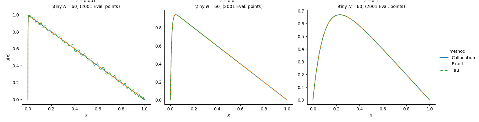
Solution comparison

Compare Tau and Collocation solutions across different boundary layer widths.

N = df_sol["N"].iloc[0]
n_eval_points = df_sol["x"].nunique()

g = sns.relplot(
    data=df_sol,
    x="x",
    y="u",
    hue="method",
    style="method",
    kind="line",
    col="eps",
    col_wrap=3,
    facet_kws=dict(sharey=False, sharex=True),
    height=4,
    aspect=1.2,
)
g.set_axis_labels(r"$x$", r"$u(x)$")
g.figure.suptitle(r"Tau vs Collocation", y=1.05)
g.set_titles(
    r"$\varepsilon={col_name:g}$"
    + "\n"
    + rf"\tiny $N = {N}$, ({n_eval_points} Eval. points)"
)

output = save_dir / "solutions_facet.pdf"
g.figure.savefig(output, bbox_inches="tight")
print(f"  Saved: {output}")

Saved: /home/docs/checkouts/readthedocs.org/user_builds/02689-advanced-num-alg/checkouts/latest/figures/A2/ex_a/solutions_facet.pdf

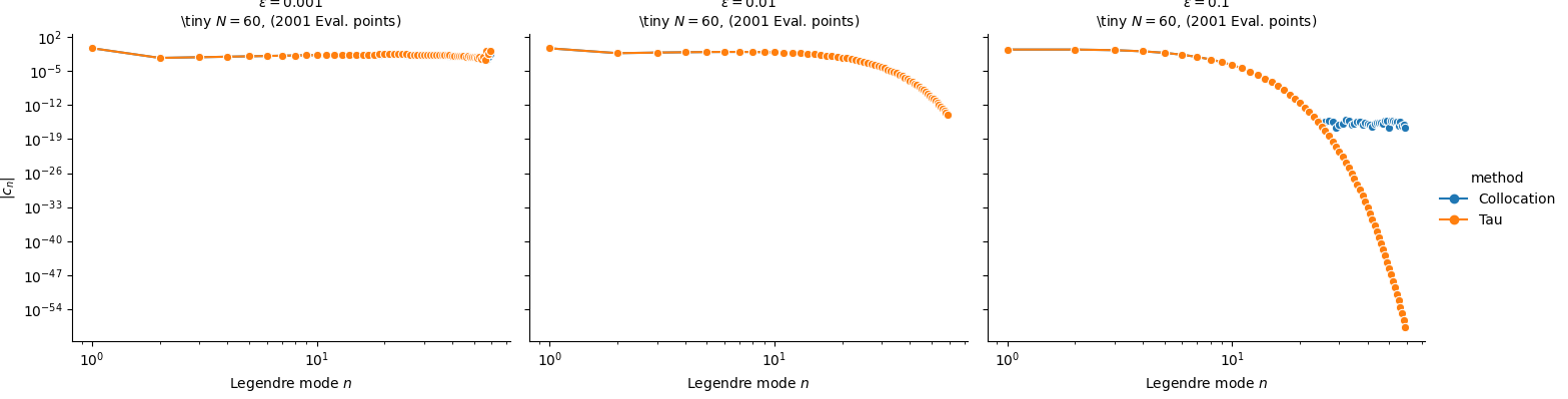
Coefficient decay

Visualize how Legendre coefficients decay for both methods.

df_coef = df[df["data_type"] == "coefficient"]
df_coef2 = df_coef[df_coef["method"] != "Exact"]

# Filter out mode 0 for log scale
df_coef_plot = df_coef2[df_coef2["mode"] > 0].copy()
df_coef_plot["method"] = df_coef_plot["method"].cat.remove_unused_categories()


g2 = sns.relplot(
    data=df_coef_plot,
    x="mode",
    y="abs_coeff",
    hue="method",
    style="method",
    kind="line",
    col="eps",
    col_wrap=3,
    marker="o",
    dashes=False,
    height=4,
    aspect=1.2,
)
g2.set(xscale="log", yscale="log", xlabel=r"Legendre mode $n$", ylabel=r"$|c_n|$")
g2.figure.suptitle(r"Tau vs Collocation", y=1.05)
g2.set_titles(
    r"$\varepsilon={col_name:g}$"
    + "\n"
    + rf"\tiny $N = {N}$, ({n_eval_points} Eval. points)"
)

output = save_dir / "coefficients_facet.pdf"
g2.figure.savefig(output, bbox_inches="tight")
print(f"  Saved: {output}")

Saved: /home/docs/checkouts/readthedocs.org/user_builds/02689-advanced-num-alg/checkouts/latest/figures/A2/ex_a/coefficients_facet.pdf

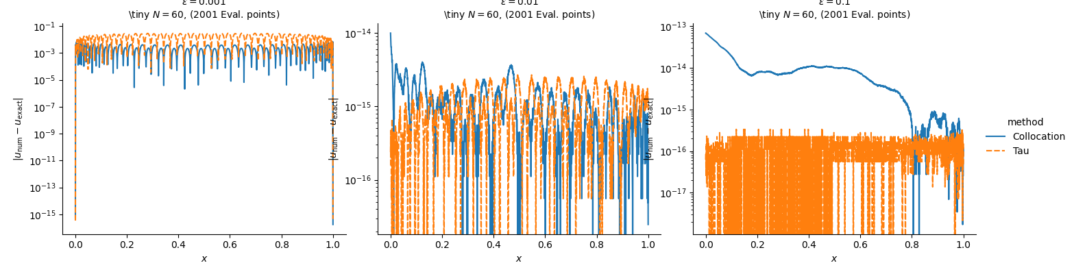
Error profiles

Show pointwise error distributions for both methods.

print("\nCreating error profiles...")
df_sol = df_sol[df_sol["method"] != "Exact"]
df_sol["method"] = df_sol["method"].cat.remove_unused_categories()

g3 = sns.relplot(
    data=df_sol,
    x="x",
    y="pointwise_err",
    hue="method",
    style="method",
    kind="line",
    col="eps",
    col_wrap=3,
    facet_kws=dict(sharey=False),
    height=4,
    aspect=1.2,
)
g3.set(yscale="log", xlabel=r"$x$", ylabel=r"$|u_{\rm num}-u_{\rm exact}|$")
g3.figure.suptitle(r"Tau vs Collocation", y=1.05)
g3.set_titles(
    r"$\varepsilon={col_name:g}$"
    + "\n"
    + rf"\tiny $N = {N}$, ({n_eval_points} Eval. points)"
)

output = save_dir / "errors_facet.pdf"
g3.figure.savefig(output, bbox_inches="tight")
print(f"  Saved: {output}")

Creating error profiles...
  Saved: /home/docs/checkouts/readthedocs.org/user_builds/02689-advanced-num-alg/checkouts/latest/figures/A2/ex_a/errors_facet.pdf

Convergence study

Analyze how error decreases with increasing number of modes.

print("\nCreating convergence plots...")
convergence_df = pd.read_parquet(data_dir / "convergence.parquet")

# Create faceted convergence plot
g4 = sns.relplot(
    data=convergence_df,
    x="N",
    y="Linf_err",
    hue="method",
    style="method",
    kind="line",
    col="eps",
    col_wrap=3,
    marker="o",
    facet_kws=dict(sharey=False),
    height=4,
    aspect=1.2,
)
g4.set(
    xscale="log",
    yscale="log",
    xlabel=r"Number of modes $N$",
    ylabel=r"$L^\infty$ Error",
)

# Add parameter info (N range varies for convergence study)
N_min = convergence_df["N"].min()
N_max = convergence_df["N"].max()

# Title hierarchy: main title and column titles with parameters
g4.figure.suptitle(r"Tau vs Collocation", y=1.05)
g4.set_titles(
    r"$\varepsilon={col_name:g}$"
    + "\n"
    + rf"\tiny $N \in [{N_min}, {N_max}]$, ({n_eval_points} Eval. points)"
)

# Add reference lines to each subplot
for ax, (eps_val, group) in zip(
    g4.axes.flat, convergence_df.groupby("eps", observed=True)
):
    N_vals = group["N"].unique()
    N_ref = np.array([N_vals.min(), N_vals.max()])

    # O(N^-2) reference line
    slope = -2
    err_ref_start = group[group["N"] == N_vals.min()]["Linf_err"].max()
    err_ref = err_ref_start * (N_ref / N_vals.min()) ** slope

    ax.plot(
        N_ref, err_ref, "k--", alpha=0.5, linewidth=1.5, label=r"$\mathcal{O}(N^{-2})$"
    )
    ax.legend()

output = save_dir / "convergence_facet.pdf"
g4.figure.savefig(output, bbox_inches="tight")
print(f"  Saved: {output}")

Creating convergence plots...
  Saved: /home/docs/checkouts/readthedocs.org/user_builds/02689-advanced-num-alg/checkouts/latest/figures/A2/ex_a/convergence_facet.pdf